
Introduction
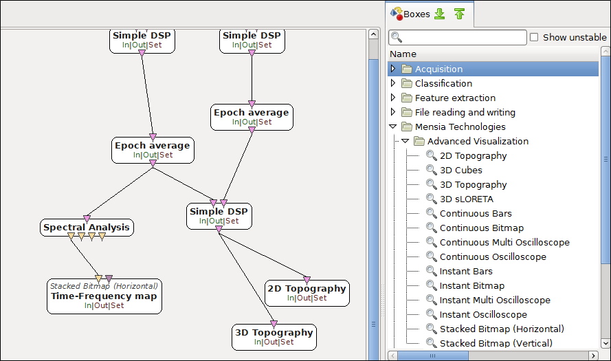
The Mensia Advanced Visualization Toolset is a collection of boxes dedicated to the visualization of the result of electrophysiological signal analysis, and are especially suitable for the real-time analysis of EEG signals , from raw signal display to 3D source reconstruction.
It addresses many different use-cases among users. Neurophysiologists can observe accurately in real-time spatial and temporal patterns in the brain activity (motor activity, cognitive processes). EEG signal processing specialists can evaluate and compare instantly algorithms effects (source separation, denoising techniques). BCI researchers can study how their ERP-based system may be tuned to elicit and detect the best brain response.
Visualization paradigms
This Toolset has been designed to be very versatile. The main design concept revolves around the data presentation. You basically want to display matrices of numbers which may have temporal, and/or spatial meanings. The most adapted data presentation may vary from one case to another, according to the type of events or patterns on which you need to get a good contrast.
Before choosing the right visualization box, ask yourself:
- How do I want my data to be displayed ? curves ? levels ?
- What will be the best way to enhance the contrast between the information I want to extract and the rest of the data ?
- Is my data stream continuous in time ? or am I dealing with discontinuous epochs (e.g. ERPs) ?
To be adapted in most situation, the Mensia Advanced Visualization Toolset has been designed to cover different visualization paradigms. Take a look at all the possibilities and choose what will best fit your needs.
You can also have a look at the list of use-cases, showing how each box can be used on concrete, real-life examples.
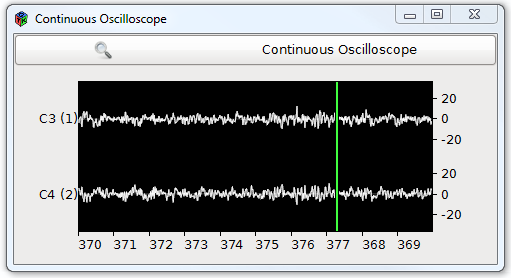
The Oscilloscope view
It is the most basic paradigm, used to display temporal numerical data in the form of curves (dots linked by lines). The Oscilloscope views are all expecting centered values (i.e. distributed around 0). Hence it is advised to use at least one temporal filter (e.g. band passing between 2 and 40 Hz using a Temporal Filter box) before displaying an EEG signal.
Four boxes use this paradigm:
- Continuous Oscilloscope box: displays continuous data from left to right on a defined horizontal scale (goes back to origin upon reaching the end of the scale), channels are displayed vertically one after another, but spikes may overlap.
- Instant Oscilloscope box: displays each block of data received as it comes, filling all the horizontal space available.
- Continuous Multi Oscilloscope box: same as the Continuous Oscilloscope, but every input channels are displayed along the same horizontal axis with a different color, additively.
- Instant Multi Oscilloscope box: same as the Instant Oscilloscope, but every input channels are displayed along the same horizontal axis with a different color, additively.
Example: raw EEG signal display.
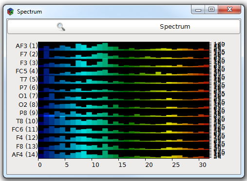
The Bar view
Like histograms, this paradigm can be used to display and compare series of levels . Levels are displayed one after another from left to right, within a color gradient . Channels are displayed vertically, one after another with a fixed interval (thus some "high" levels may overlap). With a high definition (i.e. a rather high frequency display), the result can be viewed as a curve colored below the line.
Two boxes uses this paradigm:
- Continuous Bars box: displays continuous data from left to right on a defined horizontal scale (goes back to origin upon reaching the end of the scale).
- Instant Bars box: displays each block of data received as it comes, filling all the horizontal space.
Example: spectrum display.
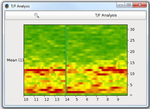
The Bitmap view
The bitmap paradigm displays matrices of data using a color gradient. The result is a 2D map where each cell is given a color "bit" . This view using colors can enhance easily the constrast between 2 temporal or spatial patterns, as the difference between "cold" and "hot" colors is quickly caught by the analyst's eye. You can even add an additional dimension by using stacked bitmaps : every time a new bitmap is received, it is placed on top or left to the previous one.
Four boxes uses this paradigm:
- Continuous Bitmap box: displays continuous data from left to right on a defined horizontal scale (goes back to origin upon reaching the end of the scale).
- Instant Bitmap box: displays each block of data received as it comes, filling all the horizontal space.
- Stacked Bitmap (Vertical) box: each bitmap is placed on top of the previous one.
- Stacked Bitmap (Horizontal) box: each bitmap is placed left to the previous one.
Example: Time-frequency map.
The Topographic view
This paradigm adds a strong spatial constraint on the input data: each channel must be labelled with an electrode name in a defined nomenclature, such as the standard 10-20 system. Please see Channel localization for further details.
Here again the data itself is displayed using a color gradient, mapped to a 2D or 3D model using spherical spline interpolation. For more details about the spherical spline interpolation, please check F. Perrin, J. Pernier, O. Bertrand, J.F. Echallier, Spherical splines for scalp potential and current density mapping, Electroencephalography and Clinical Neurophysiology, Volume 72, Issue 2, February 1989, Pages 184-187.
The 2D model is a planar projection of the scalp, covering the scalp roughly from the frontal area to the occipital area (i.e. from Fp1-Fp2 to O9-O10 sites). The projection result takes the shape of a disk with a crescent growth at the back for the occipital region.
Three boxes uses this paradigm:
- 2D Topography box: maps the input (which channels are labelled in the 10-20 system standard) to a planar projection of the scalp.
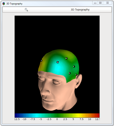
- 3D Topography box: maps the input (which channels are labelled in the 10-20 system standard) to a projection on a 3D model of the scalp.
- 3D Cubes box: an alternative view where each channel is represented by a 3D cube, positionned in space as the electrode would be on the 3D model. The activity is rendered by changing the size and color of the cubes.
Example: Displaying the power of a specific frequency band on a 3D head model.
The Reconstruction view
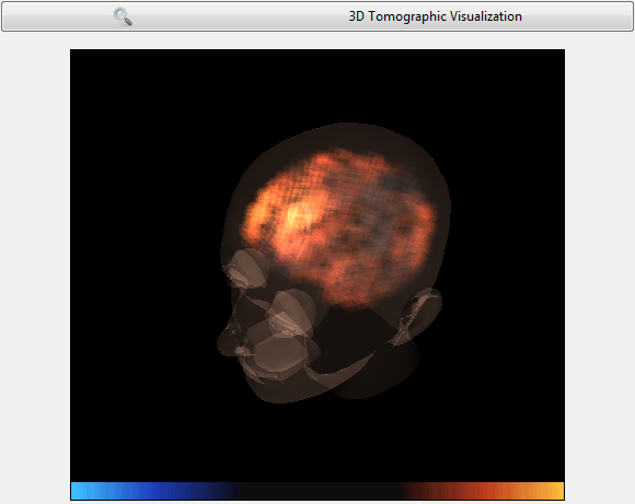
Tomographic reconstruction algorithms offer an inside look, into the brain, from only surface measurements. Several techniques exist, including the algorithms of the popular LORETA family which slice the brain in a stack of little cubes called voxels, and computes the inverse model, a model reconstructing the sources of the potentials acquired at the measurement site.
One box implements the source reconstruction view:
- Doc_BoxAlgorithm_3DSourceVisualization box : displays a 3D source reconstruction using 2394 colored/translucent voxels in a 3D head model. This box expects 2394 input channels, produced by an inverse model (i.e. a spatial filter with N sensor inputs for 2394 sources outputs). This model must be tailor-made for the precise EEG setup being used (e.g. using sLORETA).
Channel localization
Every visualization box can use the spatial information conveyed by the electrode naming. The channels can be positionned relatively to each other as long as you provide in the box settings a file containing the cartesian coordinates of the electrodes. Most of the time, EEG manufacturers use the 10-20 system as an electrode naming standard. For convenience, we provide within the Toolset a file compiling all the coordinates of the electrodes in the 10-20 system.
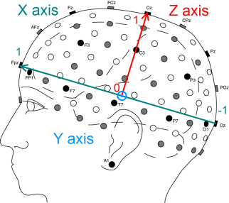
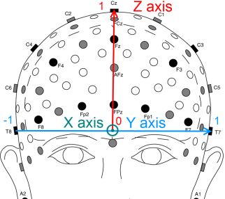
The cartesian coordinates of all the electrodes are computed in the 3D space, where the origin is at the center of [Fpz,Oz] and [T7,T8].
- the X axis goes from the occipital lobe to the frontal lobe
- the Y axis goes from the right temporal lobe to the left temporal lobe
- the Z axis goes from the center of the head to the top
And as for the unit, here are some key points at the maximum of the axis:
- Fpz (1,0,0)
- Oz (-1,0,0)
- T7 (0,1,0)
- T8 (0,-1,0)
- Cz (0,0,1)
The following figures illustrates the cartesian coordinates of the extended 10-20 system used in the Mensia Advanced Visualization Toolset.
For more information, please see Oostenveld, R. & Praamstra, P. (2001). The five percent electrode system for high-resolution EEG and ERP measurements. Clinical Neurophysiology, 112:713-719
Please note that using the 10-20 system is not mandatory. To use all the Toolset features related to the spatial disposition of the electrodes, you just need to provide a file that maps electrode name with their coordinates in the space described above.
The format of this file is simple text. You must provide:
- the electrode names as a list of quoted labels
- the coordinate system labels
- the electrode coordinates of the electrodes, in the same order as in the electrode names
For example:
For a complete example, please look at the file provided with the Toolset (../share/mensia /openvibe-plugins/cartesian.txt)
Generated on Tue Jun 26 2012 15:25:54 for Documentation by
 1.7.4
1.7.4