Continuous Multi Oscilloscope

Summary

• Plugin name : Continuous Multi Oscilloscope
• Version : 1.0
• Author : Yann Renard
• Company : Mensia Technologies SA
• Short description : Displays the input matrices as a series of curves. All channels are rendered on the same vertical axis, with different colors.
• Documentation template generation date : Jan 9 2018

Description

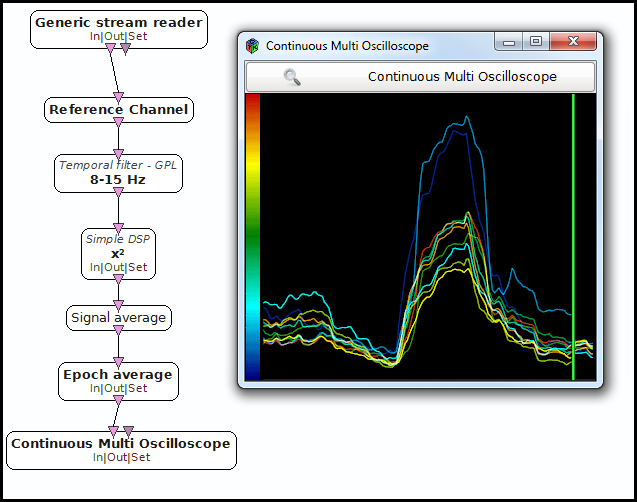
The Continuous Multi-Oscilloscope displays temporal numerical data in the form of curves, on the same vertical axis. Each channel is given a color according to a color gradient, rendered additively. The display is done continuously , meaning that once the end of the horizontal scale is reached, it goes back to the origin.

The Continuous Multi-Oscilloscope box shares common concepts and settings with the other boxes in the Mensia Advanced Visualization Toolset . Additional information are available in the dedicated documentation pages:

• Concepts
• Configuration

Inputs

1. Matrix

The first input can be a streamed matrix or any derived stream (Signal, Spectrum, Feature Vector). Please set the input type according to the actual stream type connected.

• Type identifier : Signal (0x5ba36127, 0x195feae1)

2. Markers

The second input expect stimulations. They will be displayed as red vertical lines .

• Type identifier : Stimulations (0x6f752dd0, 0x082a321e)

Settings

1. Channel Localisation

The channel localisation file containing the cartesian coordinates of the electrodes to be displayed. A default configuration file is provided, and its path stored in the configuration token ${AdvancedViz_ChannelLocalisation}.

• Type identifier : Filename (0x330306dd, 0x74a95f98)
• Default value : [ ${AdvancedViz_ChannelLocalisation} ]

2. Temporal Coherence

Select Time Locked for a continuous data stream, and specify the time scale below. Select Independent for a discontinuous data stream, and specify the matrix count below.

• Type identifier : Temporal Coherence (0x8f02e3f6, 0xffb00f4b)
• Default value : [ Time Locked ]

3. Time Scale

The time scale in seconds, before the displays goes back to the origin.

• Type identifier : Float (0x512a166f, 0x5c3ef83f)
• Default value : [ 20 ]

4. Matrix Count

The number of input matrices to receive before the displays goes back to the origin.

• Type identifier : Integer (0x007deef9, 0x2f3e95c6)
• Default value : [ 50 ]

5. Positive Data Only ?

If this checkbox is ticked, the vertical scale is shifted so that 0 is at the bottom. Only positive values will be displayed.

• Type identifier : Boolean (0x2cdb2f0b, 0x12f231ea)
• Default value : [ false ]

6. Gain

Gain (floating-point scalar factor) to apply to the input values before display.

• Type identifier : Float (0x512a166f, 0x5c3ef83f)
• Default value : [ 1 ]

7. Caption

Label to be displayed on top of the visualization window.

• Type identifier : String (0x79a9edeb, 0x245d83fc)
• Default value : [ ]

8. Translucency

This setting expect a value between 0 and 1, from transparent to opaque color rendering (nb: this value is the alpha component of the color).

• Type identifier : Float (0x512a166f, 0x5c3ef83f)
• Default value : [ 1 ]

9. Color

Color gradient to use. This setting can be set manually using the color gradient editor. Several presets exist in form of configuration tokens ${AdvancedViz_ColorGradient_X}, where X can be:

• Matlab or Matlab_Discrete
• Icon or Icon_Discrete
• Elan or Elan_Discrete
• Fire or Fire_Discrete
• IceAndFire or IceAndFire_Discrete

The default values AdvancedViz_DefaultColorGradient or AdvancedViz_DefaultColorGradient_Discrete are equal to </t>Matlab and Matlab_Discrete.

An example of topography rendering using these color gradients can be found here.

• Type identifier : (0x3d3c7c7f, 0xef0e7129)
• Default value : [ ${AdvancedViz_DefaultColorGradient} ]

Examples

In the following example, we compute the band power of the input signal in the 8-15 Hz frequency range, and average it over the last 32 epochs received.

You can find a commented scenario in the provided sample set, the scenario file name is {ContinuousMultiOscilloscope.mxs}.

Example of scenario using the Continuous Multi-Oscilloscope

Miscellaneous